R からシームレスに Python を呼べる reticulate が便利だった

t2sy

2018.4.13

Topics

reticulate パッケージのインストール
Python REPL
Sourcing Python scripts
おわりに

こんにちは。データサイエンスチームの t2sy です。
この記事では、R と Python をシームレスに繋ぐことができる reticulate パッケージを紹介します。
reticulate パッケージを使うことで R を主に使っているデータ分析者が、分析の一部で Python を使いたい場合に R からシームレスに Python を呼ぶことができ、ワークフローの効率化が期待できます。
実行環境は以下です。

Amazon EC2: t2.large インスタンス (vCPU: 2, メモリ: 8GiB)
Ubuntu Server: 16.04 LTS
RStudio Server: 1.1.442
Anaconda: 2-5.1.0
scikit-learn: 0.19.1
umap-learn: 0.2.1

 > sessionInfo()
 R version 3.4.4 (2018-03-15)
 Platform: x86_64-pc-linux-gnu (64-bit)
 Running under: Ubuntu 16.04.4 LTS
 Matrix products: default
 BLAS: /usr/lib/libblas/libblas.so.3.6.0
 LAPACK: /home/t2sy/anaconda2/lib/libmkl_rt.so

reticulate パッケージのインストール

reticulate パッケージは R コンソールから install.packages() でインストールできます。

 > install.packages("reticulate")

reticulate で Python を R から利用するには以下の方法があります。

Python in R Markdown
Importing Python modules
Python REPL
Sourcing Python scripts

今回は Python REPL と Sourcing Python scripts について紹介します。

Python REPL

repl_python() により R から Python REPL を呼ぶことができます。以下は Python2 ですが Python3 でも動作します。

 > library(reticulate)
 > use_condaenv("/home/t2sy/anaconda2/bin")
 >
 > repl_python()
 Python 2.7.14 (/home/t2sy/anaconda2/bin/python)
 Reticulate 1.6 REPL -- A Python interpreter in R.
 >>>
 >>> import pandas as pd
 >>> from sklearn import datasets
 >>>
 >>> boston = datasets.load_boston()
 >>> X = pd.DataFrame(boston.data, columns=boston.feature_names)
 >>> y = pd.DataFrame(boston.target, columns=["MEDV"])
 >>>
 >>> df = pd.concat([X, y], axis=1)
 >>> type(df)
 <class 'pandas.core.frame.DataFrame'>
 >>> df.head()
 CRIM    ZN  INDUS  CHAS    NOX     RM   AGE     DIS  RAD    TAX
 0  0.00632  18.0   2.31   0.0  0.538  6.575  65.2  4.0900  1.0  296.0
 1  0.02731   0.0   7.07   0.0  0.469  6.421  78.9  4.9671  2.0  242.0
 2  0.02729   0.0   7.07   0.0  0.469  7.185  61.1  4.9671  2.0  242.0
 3  0.03237   0.0   2.18   0.0  0.458  6.998  45.8  6.0622  3.0  222.0
 4  0.06905   0.0   2.18   0.0  0.458  7.147  54.2  6.0622  3.0  222.0
 PTRATIO       B  LSTAT  MEDV
 0     15.3  396.90   4.98  24.0
 1     17.8  396.90   9.14  21.6
 2     17.8  392.83   4.03  34.7
 3     18.7  394.63   2.94  33.4
 4     18.7  396.90   5.33  36.2
 >>> exit

Python REPL 内のオブジェクトは reticulate により Python のデータ型から R のデータ型に変換され py オブジェクトに格納されます。R 側では py オブジェクトから $ 演算子を使いアクセスすることができます。

 > df = py$df
 > class(df)
 [1] "data.frame"
 > head(df)
 CRIM ZN INDUS CHAS   NOX    RM  AGE    DIS RAD TAX PTRATIO      B LSTAT MEDV
 1 0.00632 18  2.31    0 0.538 6.575 65.2 4.0900   1 296    15.3 396.90  4.98 24.0
 2 0.02731  0  7.07    0 0.469 6.421 78.9 4.9671   2 242    17.8 396.90  9.14 21.6
 3 0.02729  0  7.07    0 0.469 7.185 61.1 4.9671   2 242    17.8 392.83  4.03 34.7
 4 0.03237  0  2.18    0 0.458 6.998 45.8 6.0622   3 222    18.7 394.63  2.94 33.4
 5 0.06905  0  2.18    0 0.458 7.147 54.2 6.0622   3 222    18.7 396.90  5.33 36.2
 6 0.02985  0  2.18    0 0.458 6.430 58.7 6.0622   3 222    18.7 394.12  5.21 28.7

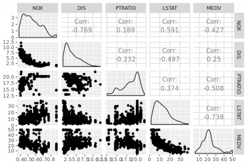
上記の通り Pandas DataFrame は R の data.frame に変換されることが確認できました。せっかくなので、得られた data.frame を ggplot2 (GGally) でプロットしてみます。

 > library(dplyr)
 > library(GGally)
 > df %>%
 + select(NOX, DIS, PTRATIO, LSTAT, MEDV) %>%
 + ggpairs()

Sourcing Python scripts

source_python() にファイル名を指定することで Python のソースコードを R から呼ぶことができます。
今回は例として、以下の2つのデータセットに対し可視化・次元削減手法 UMAP と t-SNE の実行を Python で行い、埋め込み結果を R でプロットしてみます。

MNIST: 0-9 の手書き数字画像に対応するラベルが関連付けられたデータセット
Fashion MNIST: ファッション画像に対応する10クラスからのラベルが関連付けられたデータセット

UMAP は t-SNE と同程度の可視化の質 (visualization quality) を持ちつつも、高速でスケーラブルな可視化・次元削減手法です。UMAP のアルゴリズムの詳細については arXiv に投稿されている論文を参照ください。
R から呼ぶ Python コードは以下です。

import sys
sys.path.append("./fashion-mnist/utils")
import time
import mnist_reader
import umap
import numpy as np
from sklearn import datasets
from sklearn.manifold import TSNE
def load_mnist():
  digits = datasets.fetch_mldata('MNIST original')
  return digits.data/255.0, digits.target
def load_fmnist(path):
  train_X, train_y = mnist_reader.load_mnist(path, kind='train')
  test_X, test_y = mnist_reader.load_mnist(path, kind='t10k')
  X = np.concatenate((train_X, test_X), axis=0)
  y = np.concatenate((train_y, test_y), axis=0)
  return X, y
def timeit(X, func, **kwargs):
  start = time.time()
  embedding = func(**kwargs).fit_transform(X)
  end = time.time()
  return embedding, end-start
def embed(dataset, method, path=""):
  if dataset == "mnist":
    X, y = load_mnist()
  elif dataset == "fmnist":
    X, y = load_fmnist(path)
  else:
    return "Unknown dataset"
  if method == "tsne":
    embedding, diff = timeit(X, TSNE, n_components=2)
  elif method == "umap":
    embedding, diff = timeit(X, umap.UMAP)
  else:
    return "Unknown embedding method"
  return {"embedding": embedding, "labels": y, "time": diff}

embed() の戻り値は Dict 型で R に渡されるときに Named list に変換されます。
R のコードは以下です。 source_python() で上記の Python コードを読み込んだ後は、Python の関数を通常の R 関数のように呼ぶことができます。

library(tibble)
library(dplyr)
library(ggplot2)
library(reticulate)
use_condaenv("/home/t2sy/anaconda2/bin")
source_python("embedding.py")
plot_point <- function(df, color, title, label_name) {
  ggplot(df, aes(x = V1, y = V2, colour = color)) +
    geom_point(size = 0.75) +
    labs(title = title, x = "", y = "") +
    scale_colour_discrete(name = label_name)
}
# MNIST Digits Embedded via UMAP
res <- embed("mnist", "umap")
print(res$time)
g <- plot_point(as_tibble(res$embedding),
                color = as.factor(res$labels),
                title = "MNIST Digits Embedded via UMAP",
                label_name = "Digits")
plot(g)
# MNIST Digits Embedded via t-SNE
res2 <- embed("mnist", "tsne")
print(res2$time)
g2 <- plot_point(as_tibble(res2$embedding),
                 color = as.factor(res2$labels),
                 title = "MNIST Digits Embedded via t-SNE",
                 label_name = "Digits")
plot(g2)
# Fashion MNIST Embedded via UMAP
fmnist_desc <- data.frame(label = c(0:9),
                          description = as.factor(c("T-shirt/top", "Trouser", "Pullover",
                                                    "Dress", "Coat", "Sandal", "Shirt",
                                                    "Sneaker", "Bag", "Ankle boot")))
res3 <- embed("fmnist", "umap", "./fashion-mnist/data/fashion")
print(res3$time)
fmnist_label <- data.frame(label = res3$labels) %>%
  left_join(fmnist_desc, by = "label")
g3 <- plot_point(as_tibble(res3$embedding),
                 color = fmnist_label$description,
                 title = "Fashion MNIST Embedded via UMAP",
                 label_name = "Label")
plot(g3)
# Fashion MNIST Embedded via t-SNE
res4 <- embed("fmnist", "tsne", "./fashion-mnist/data/fashion")
print(res4$time)
g4 <- plot_point(as_tibble(res4$embedding),
                 color = fmnist_label$description,
                 title = "Fashion MNIST Embedded via t-SNE",
                 label_name = "Label")
plot(g4)

MNIST を UMAP と t-SNE で2次元に埋め込んだ結果は以下となりました。

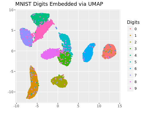
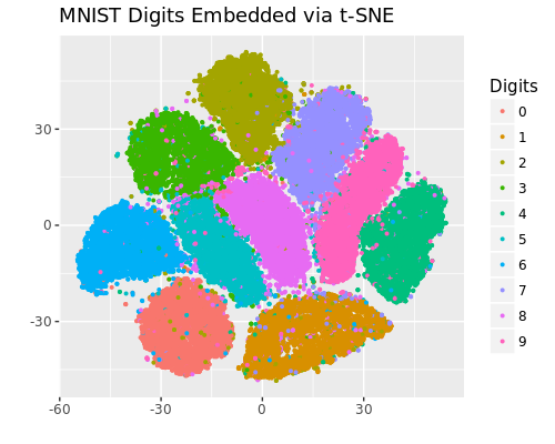
どちらの結果も概ね綺麗に10個のクラスタに分かれており、構造を保持したまま2次元に埋め込まれています。
Fashion MNIST を UMAP と t-SNE で2次元に埋め込んだ結果は以下となりました。

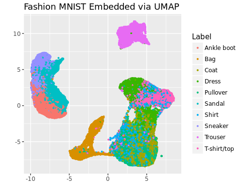
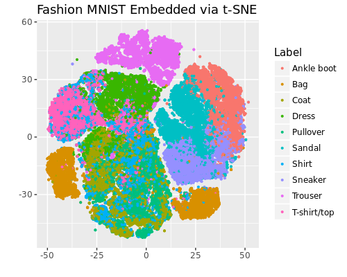
どちらの結果も Sandal, Ankle boot, Sneaker といった履物や Trouser、 Bag が独立したクラスタを形成しています。さらに、UMAPは大域的な構造も保持していることが窺えます。
続いて、実行時間 (3回の平均値) を確認してみます。t-SNE は scikit-learn 実装を使用しており、 t-SNE の論文著者による C++ を用いた高速な実装 bhtsne との比較ではない点にご注意下さい。

DataSet	DataSet Size	UMAP	t-SNE (scikit-learn)
MNIST	70,000 x 784	145.18 s	9000.90 s
Fashion MNIST	70,000 x 784	155.24 s	9240.58 s

MNIST、 Fashion MNIST に対して UMAP は t-SNE (scikit-learn) に比べ 60 倍程度高速であることがわかります。

おわりに

この記事では reticulate パッケージをご紹介しました。冒頭にも触れたように reticulate パッケージを使うことで R からシームレスに Python を呼ぶことができ、ワークフローの効率化が期待できます。
余談になりますが、私が reticulate パッケージを使おうと思ったきっかけは scikit-learn の API が統一的で使いやすいと感じる一方で Python の可視化ライブラリ Matplotlib や Seaborn などに慣れていないため、 R の ggplot2 でプロットしたいということでした。
▽NHN テコラスではいまからはじめるデータ活用・分析相談会を行っております。データ分析に関する技術的なお悩みにも個別にお答えしています。参加は無料なので、お気軽にお申し込みください。